Cascading Data Validation Lists

..with thanks to  Melodie S. for her help with this post.

A dear associate of mine asked for assistance with the following: How can you dynamically link a validation list, so that choices in one column control the list displayed in another?

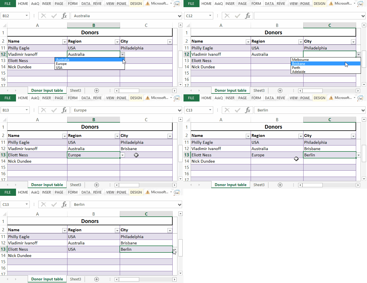
Cascading Data Validation Lists3

The example above illustrates a Region – City validation list. The selection of USA in the Region column will display only U.S. Cities; selecting Europe will display only European ones.

The first step is to create Defined Names for the Regions and each of the City groups.
Cascading List - Named Ranges

Creating Defined Names:

  1. Select the cells that make up the list. Do not include the list header in your selection.
    For example, to create the Region list in the above example, select E3:E5. 
  2. Click in the Name Drop-down.
  3. Type a name for the list and press Enter.
    Note: Names must begin with a letter and should not include spaces.
  4. Repeat steps 1-3 for each list (i.e., USA, Europe, Australia).

=INDIRECT(ref): Returns the reference specified by a text string.

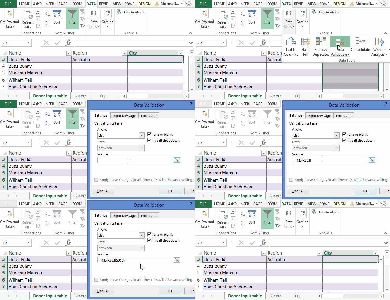
Using the INDIRECT function to reference the value in the Region column (e.g, Australia), the data validation list will display contents of the matching defined name (e.g., Brisbane, Perth, etc.)

cascading list validation dialogs

Creating the Data Validation Lists:

  1. For the first input column (e.g., Region) select the the cells where data will be input (e.g., B3:B15).
  2. On the Data tab, in the Data Tools group, click Data Validation. The Data Validation dialog appears.
  3. Click the Allow drop-down and select List.
  4. In the Source field type ‘=‘ followed by the appropriate Defined Name (i.e., =Region )
  5. Click OK.
  6. For the second input column (e.g., City) select the the cells where data is to be input (e.g., C3:C15).
  7. On the Data tab, in the Data Tools group, click Data Validation. The Data Validation dialog appears.
  8. Click the Allow drop-down and select List.
  9. Click in the Source field, type ‘=INDIRECT( ref ), where ref is the cell reference of the first Input cell in the prior column; e.g., =INDIRECT(B3) .
  10. Click OK.

Cheers!

hɔuᴉnb

Additional reading:
Windows Emoji Keyboard

In this, my last post honoring World Emoji Day (promise), I showcase the emojis available with Windows Touch Keyboard.

In addition to the new emojis in GMail, and the hidden emojis in Skype, did you know that you can access emojis using Windows’ on-screen keyboard?

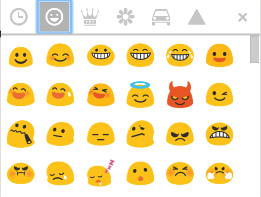
The on-screen keyboard (aka, Touch Keyboard), available to Windows desktop since versions 8, includes emoji characters similar to those used on iPhones and iPads.

emoji keyboard2

Accessing Emojis Using Windows Touch Keyboard

  1. In Desktop mode, RIGHT+CLICK on the taskbar, point to Toolbars and select Touch Keyboard. The Touch Keyboard icon TouchKeyboard Icon. now appears on the Taskbar.
  2. Click (or tap, if using a tablet) the Touch Keyboard icon to display an onscreen keyboard.
  3. Click the emoji key Emoji button_66 to display emojis.
    emojiKeyboard
  4. Click the desired emoji. That emoji is inserted at the current cursor position.

Press ‘X‘ to close the Touch Keyboard when done.

Cheers!

Additional reading:

Skype’s Hidden Emojis

This month we celebrate World Emoji Day (seriously, it’s a thing) . Last post I showcased GMail’s new emojis. Now I highlight Skype‘s emoji offerings.

Disney/Pixar Emoji’s

What better way to share you emotions than with the eponymous animated character from the movie Inside Out

PixarSkype emojis

Hidden Skype Emoji’s (shhhh…)

Although these emojis don’t appear on the menu they are available by entering the secret code (in parentheses)

For example, type (gift) into the SMS field (include the parentheses) and press the Send Send

gift_80_anim_gif

Voila, an animated present.

Here are few others (for the full list visit Skype’s FAQ support page)

gottarun_80_anim_gif poolparty_80_anim_gif stop_80_anim_gif holdon_80_anim_gif confidential_80_anim_gif
(gottarun) (poolparty) (stop) (holdon) (confidential)

Cheers!

Additional reading:

Fitting rhinos with high-tech body cams could save them from poachers

Earlier it was Penguins; now it’s Rhinos. Read why the Rhinohorn-cam is a good idea.

Gmail Gets Hundreds Of New Themes And Emoji

Just what we all need…more emojis!

The “dreams” of Google’s AI are equal parts amazing and disturbing

“Do Androids Dream of Electric Sheep?” Philip K. Dick asked that question Ridley Scott’s “Blade Runner” did little to answer that question, but now perhaps Google has. When asked to create similar images to the ones it had cataloged, the results were amazing and provided insight into the ‘electric dreams of sheep.’

Excel Text 4 of 4: Using SUBSTITUTE to Parse Text

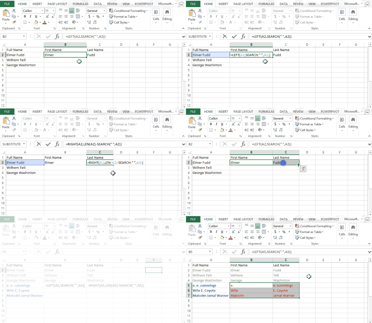
Excel is great at splitting text across multiple columns. For basic text separation (e.g. putting first and last name in separate columns) the LEFT and RIGHT functions work fine. But these functions fall short when applied to data that follow an inconsistent pattern. In the below example, the errant inclusion of a middle name wrecks havoc with our formula results.

Text4Substitute(2)

Using the SUBSTITUTE function one can identify and replace the last space in the cell with a uniquely identifying character (e.g., an underscore). This character can then be used as a delimiter to separate Lastname from full name.

ScreenShot-2015-Jun-03-126-AM

SUBSTITUTE: replace character(s) within a cell with specified character(s)

= SUBSTITUTE ( text, old text, new text, instance)
Note, instance is optional; when omitted, every occurrence of old text is replaced with the new.

Examples:

  • =SUBSTITUTE(“Mad Max”, a,i) returns Mid Mix
  • =SUBSTITUTE(“mississippi, i,“”) returns msssspp
  • =SUBSTITUTE(“banana”, a,Q”,2) returns banQna
LEN Counts the number of characters =LEN(antidisestablishmentarianism) returns 28

Click here for a 5 minute tutorial:

Cheers!

hɔuᴉnb

Additional reading: