Networkdays.INTL

As my international followers have reminded me, not every place sets aside two whole days for the weekend, nor does everyone use the same days of the week.
  • For Afghanistan, Egypt, and Pakistan their weekend starts Thursday at sunset, running from Friday through Saturday.
  • In Malaysia, based upon which part of the country your in, it’s either Saturday thru Sunday, or Friday thru Saturday.
  • Brunei Darussalam‘s non-contiguous weekend is on Friday and Sunday.
  • Costa Rica, North Korea and Uganda get only one day, Sunday, as a weekend.

As a follow-up to last week’s post here’s the international solution to calculating workdays.

NETWORKDAYS.INTL

Returns the number of whole workdays between two dates using parameters to indicate which and how many days are weekend days. Weekend days and any days that are specified as holidays are not considered as workdays.

Syntax

NETWORKDAYS.INTL(start_date, end_date, [weekend], [holidays])

  • Start_date and End_date (required). The dates for which the difference is to be computed.
  • Weekend (optional). A number value indicates the days of the week that are weekend days and are not included in the number of working. Below are the values and their corresponding weekdays.
Number Value Weekend days
1 or omitted Saturday, Sunday
2 Sunday, Monday
3 Monday, Tuesday
4 Tuesday, Wednesday
5 Wednesday, Thursday
6 Thursday, Friday
7 Friday, Saturday
11 Sunday only
12 Monday only
13 Tuesday only
14 Wednesday only
15 Thursday only
16 Friday only
17

Saturday only

Holidays (optional). Indicates the dates that are considered non working days and not counted in the number of working days.

Cheers!

hɔuᴉnb

Additional reading:


Speak Thai, Latin and Arabic with Excel.

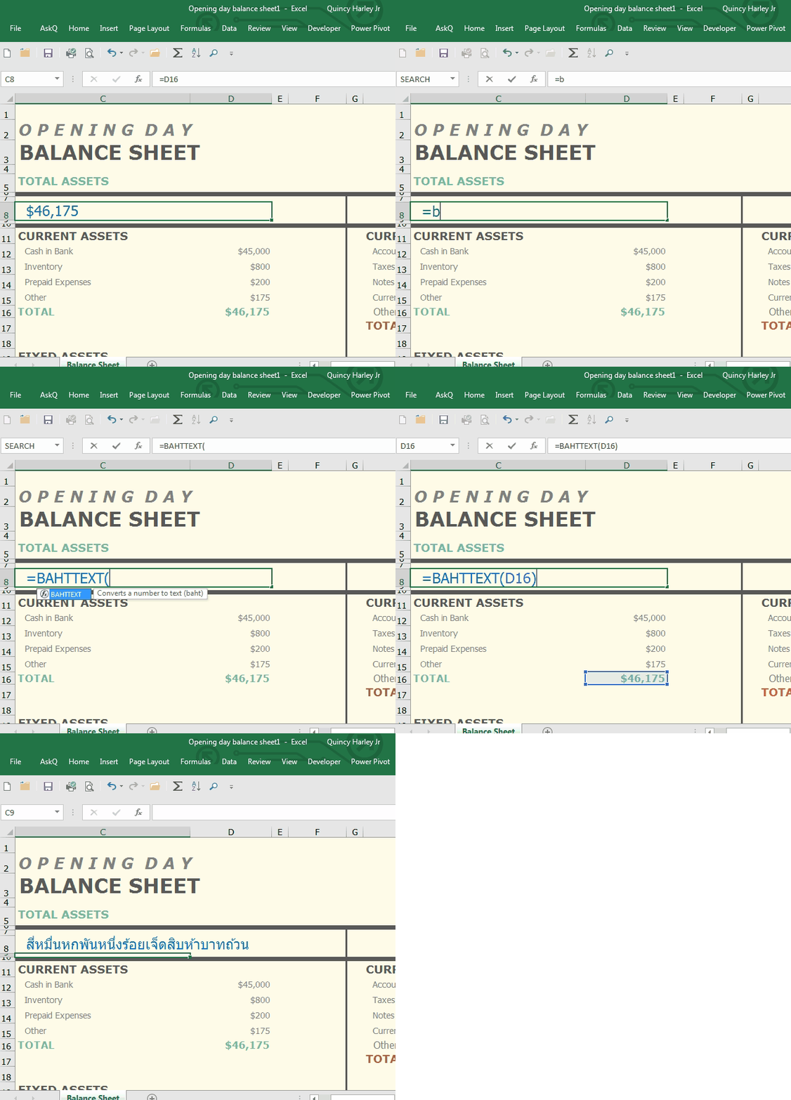
ROMAN-Starwars.gif

Ever wonder what your birthday looks like expressed in roman numerals? Want to display your travel expenses using Thai?

BAHTTEXT.gif

Use these functions to convert numbers to their respective lingo.

Formula Description Example Result
BAHTTEXT Converts number to Thai text =BAHTTEXT(451) สี่ร้อยห้าสิบเอ็ดบาทถ้วน
(Four Hundred and Fifty-one)
ARABIC Convert Roman Numeral to Arabic =ARABIC(MCDXCII) 1492
ROMAN Convert Number to Roman Numeral =ROMAN(1984 , [0] )* MCMLXXXIV

*ROMAN, has an optional argument, format . When format is included, the number is expressed differently, ranging from classic (0) to simplest (4). When this argument is omitted, the classical format is displayed.

Cheers!

hɔuᴉnb

Additional reading:

Comments and questions are always welcome!

Cascading Data Validation Lists

..with thanks to  Melodie S. for her help with this post.

A dear associate of mine asked for assistance with the following: How can you dynamically link a validation list, so that choices in one column control the list displayed in another?

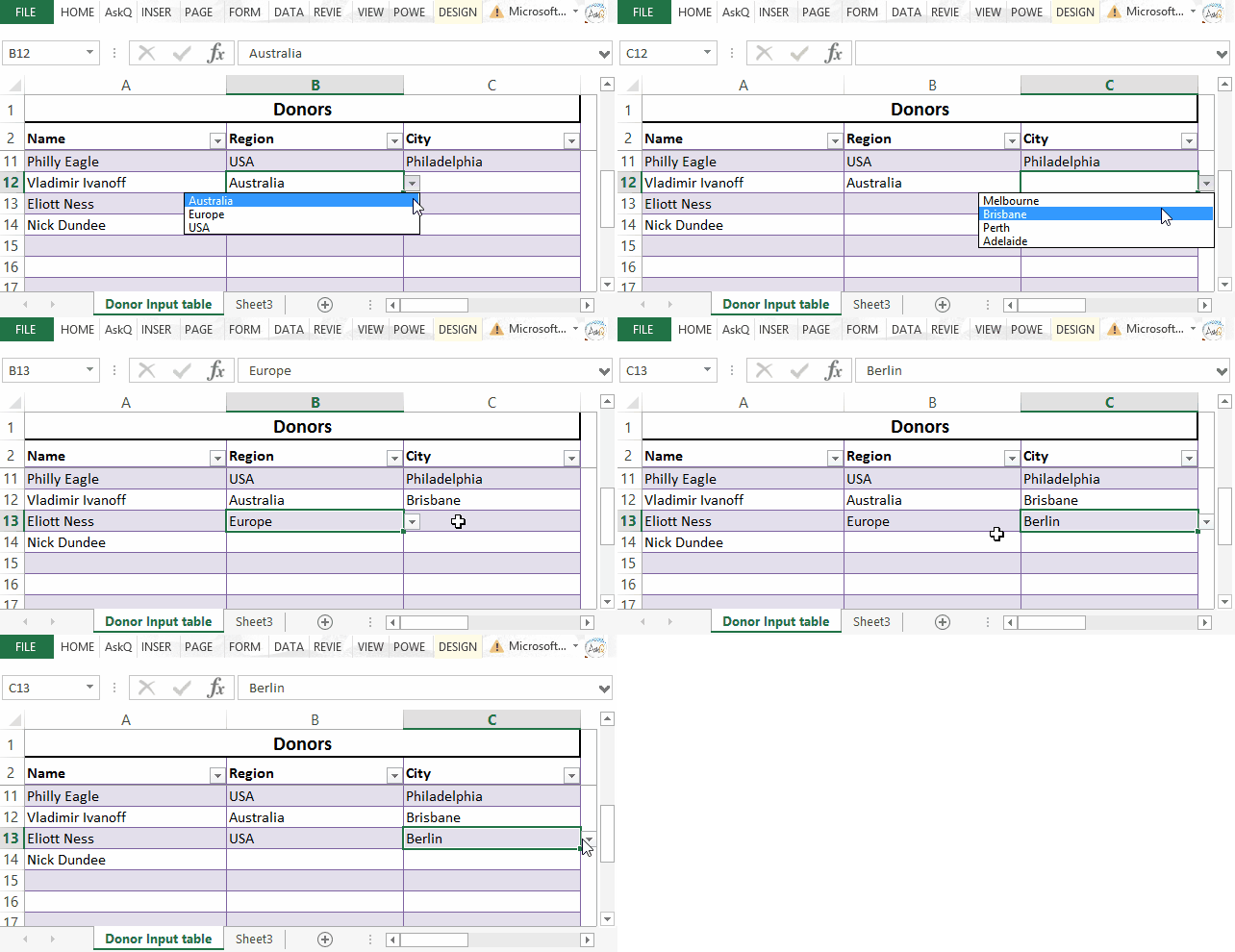
Cascading Data Validation Lists3

The example above illustrates a Region – City validation list. The selection of USA in the Region column will display only U.S. Cities; selecting Europe will display only European ones.

The first step is to create Defined Names for the Regions and each of the City groups.
Cascading List - Named Ranges

Creating Defined Names:

  1. Select the cells that make up the list. Do not include the list header in your selection.
    For example, to create the Region list in the above example, select E3:E5. 
  2. Click in the Name Drop-down.
  3. Type a name for the list and press Enter.
    Note: Names must begin with a letter and should not include spaces.
  4. Repeat steps 1-3 for each list (i.e., USA, Europe, Australia).

=INDIRECT(ref): Returns the reference specified by a text string.

Using the INDIRECT function to reference the value in the Region column (e.g, Australia), the data validation list will display contents of the matching defined name (e.g., Brisbane, Perth, etc.)

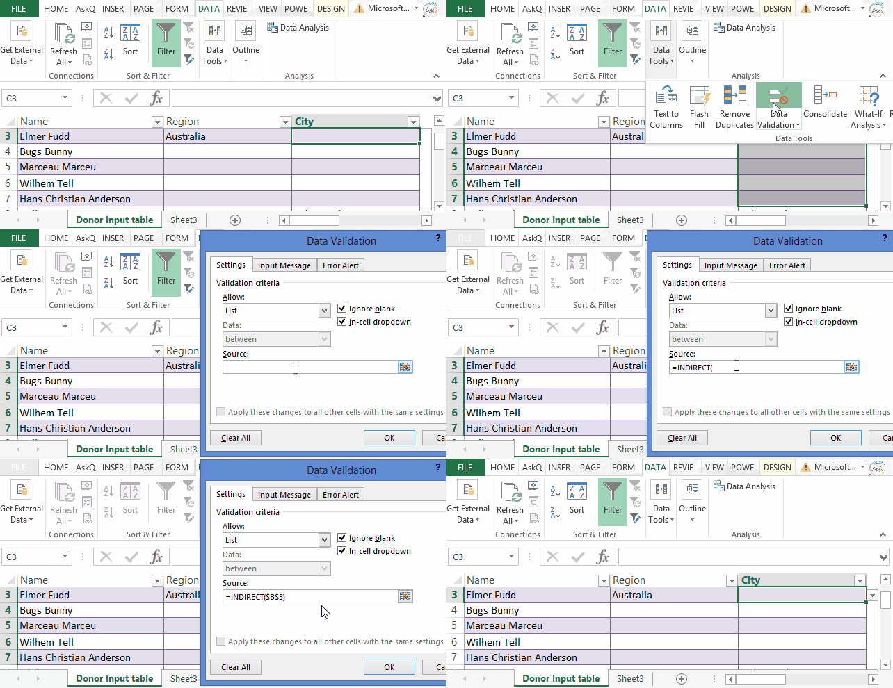
cascading list validation dialogs

Creating the Data Validation Lists:

  1. For the first input column (e.g., Region) select the the cells where data will be input (e.g., B3:B15).
  2. On the Data tab, in the Data Tools group, click Data Validation. The Data Validation dialog appears.
  3. Click the Allow drop-down and select List.
  4. In the Source field type ‘=‘ followed by the appropriate Defined Name (i.e., =Region )
  5. Click OK.
  6. For the second input column (e.g., City) select the the cells where data is to be input (e.g., C3:C15).
  7. On the Data tab, in the Data Tools group, click Data Validation. The Data Validation dialog appears.
  8. Click the Allow drop-down and select List.
  9. Click in the Source field, type ‘=INDIRECT( ref ), where ref is the cell reference of the first Input cell in the prior column; e.g., =INDIRECT(B3) .
  10. Click OK.

Cheers!

hɔuᴉnb

Additional reading:

Excel Text 4 of 4: Using SUBSTITUTE to Parse Text

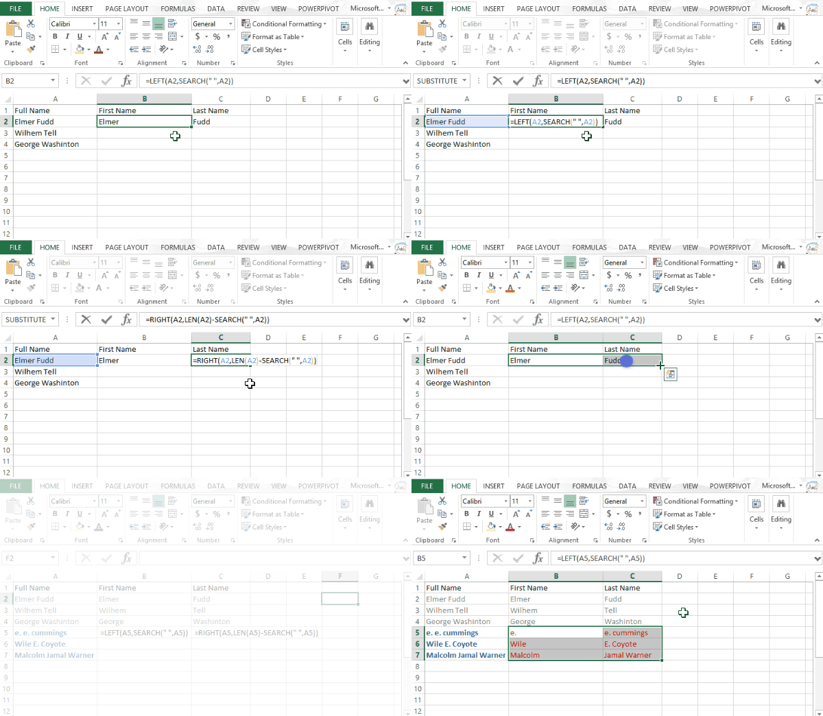
Excel is great at splitting text across multiple columns. For basic text separation (e.g. putting first and last name in separate columns) the LEFT and RIGHT functions work fine. But these functions fall short when applied to data that follow an inconsistent pattern. In the below example, the errant inclusion of a middle name wrecks havoc with our formula results.

Text4Substitute(2)

Using the SUBSTITUTE function one can identify and replace the last space in the cell with a uniquely identifying character (e.g., an underscore). This character can then be used as a delimiter to separate Lastname from full name.

ScreenShot-2015-Jun-03-126-AM

SUBSTITUTE: replace character(s) within a cell with specified character(s)

= SUBSTITUTE ( text, old text, new text, instance)
Note, instance is optional; when omitted, every occurrence of old text is replaced with the new.

Examples:

  • =SUBSTITUTE(“Mad Max”, a,i) returns Mid Mix
  • =SUBSTITUTE(“mississippi, i,“”) returns msssspp
  • =SUBSTITUTE(“banana”, a,Q”,2) returns banQna
LEN Counts the number of characters =LEN(antidisestablishmentarianism) returns 28

Click here for a 5 minute tutorial:

Cheers!

hɔuᴉnb

Additional reading:

Excel Text 3 of 4: Using SEARCH, MID & CELL to Display Sheet Name

Linking the worksheet name to a cell in the spreadsheet is easily accomplished using Excel’s CELL function. Once joined by the MID and SEARCH functions, you need only change the sheet’s name and the linked cell will update to match.

Click to view at full resolution

Displaying the Sheet Name in a Cell

Type (or copy and paste) the following formula into a cell

=MID(CELL(“filename”),SEARCH(“]”,CELL(“filename”))+1,100)

Note

  • The file must be saved; the CELL function will not return a value on an unsaved file.
  • Press F9 (if necessary) to update the cell after a renaming a sheet.
MID returns a portion of text based on starting position and number of characters. =MID(“Task Quickly”,2,5) returns “ask Q”; starting with the 2nd char, 5 charachters long.
CELL returns info about the cell, file or sheet. =CELL(“filename”) returns the path, filename and sheet.
E.g., C:\[Balance.xlsx]Sheet1
SEARCH returns  the number where the first occurrence of the search text is found, regardless of case.* =SEARCH(“A”,”Quantity”) returns 3;  ‘A’ is the 3rd character.

*The FIND function works similar to SEARCH but is case-specific.

To learn more about each function and understand why this works, watch this ~2½ minute video:

Cheers!

hɔuᴉnb

Additional reading:

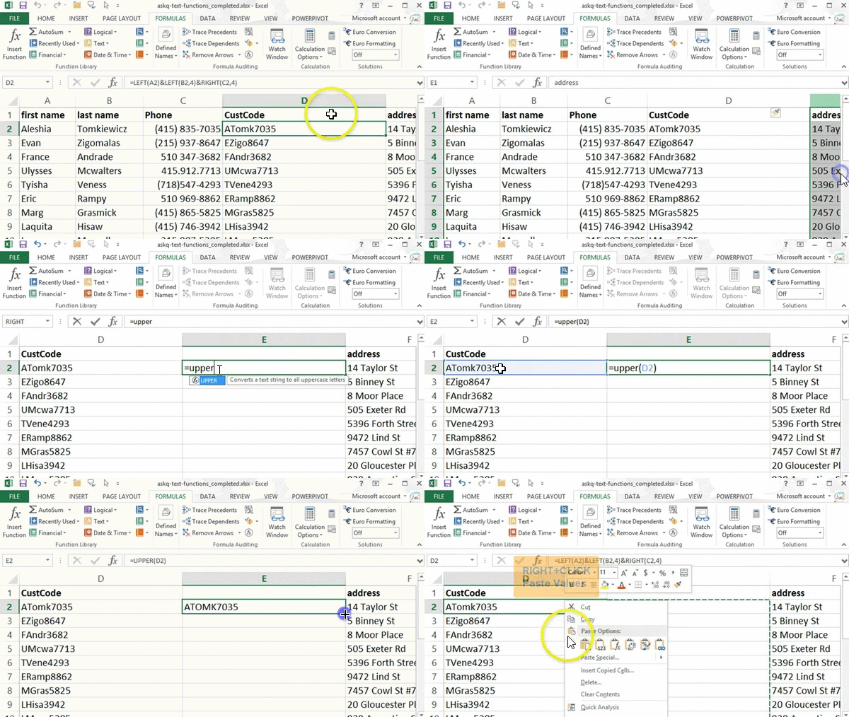
Excel Text 2 of 4: Change Case

Changing case is easily accomplished using Excel’s text functions.

Text 2-UpperCase10fps
Click to enlarge image
UPPER convert to upper case =UPPER(“Kanye”) returns KANYE
LOWER convert to lowercase =LOWER(“KIM”) returns kim
PROPER convert 1st  letter of each word to uppercase =PROPER(“north west”) returns North West

Convert Text to Uppercase

  1. In a blank cell enter =UPPER( text ), where text refers to the cell containing text to reformat. A copy is created in uppercase.
  2. Select the newly created copy and press CTRL+C (Copy).
  3. Select original cell.
  4. RIGHT+CLICK and select PASTE VALUES.

For 45 second video, click here:

Cheers!

hɔuᴉnb

Additional reading:

Excel Text Functions 1 of 4: =LEFT() and =RIGHT()

For 60 second video, click here:

During the next series of posts I will demonstrate some commonly used Text functions. In the illustrated example we populate a CustomerCode column by combining

  • the first letter of the first name,
  • the first 4 letters of the last name, and
  • the last 4 digits of the phone number

=LEFT

Returns the leftmost character(s) of a cell, as specified by the optional Num_chars argument.

LEFT Right Functions_left 4d
click image to view at full resolution


Using the LEFT function to copy the leftmost characters of a cell

  1. Select cell to display the result.
  2. On the Formulas tab, in the Function Library group, click Text drop-down and select LEFT.
  3. In Text field select or type cell containing text.
  4. In the Num_chars field enter the number of characters to copy. When left blank the result is only the leftmost character.
  5. Click OK.

Concatenate using ‘&’

Use the Ampersand (&) to concatenate (combine) text. For example, with “North” in A1 and “West” in B1, the formula =A1&B1 returns “NorthWest”

=RIGHT

Returns the rightmost character(s) of a cell, as specified by the optional Num_chars argument.

Using the RIGHT function to copy rightmost character(s) of a cell

  1. Select cell to display the result.
  2. On the Formulas tab, in the Function Library group, click Text drop-down and select RIGHT.
  3. In Text field select or type cell containing text.
  4. In the Num_chars field enter number of characters to copy. When left blank the result is only the rightmost character.
  5. Click OK.

Cheers!

hɔuᴉnb

Additional reading:

Comments and questions are always welcome!

%d bloggers like this: