Excel: Using Conditional Formatting to Highlight an Entire Row

Conditional Formatting a Row

Conditional Formatting makes it easy to visually highlight cells, based upon conditions (criteria) that you set. The conditional formats are dynamic, so as the data is edited, the criteria is tested, and the formats reapplied.

In a prior post, I mentioned how you can format an entire row or record based upon criteria found in one of that row’s fields.  Here’s the step by step example, using the Charity Guest List data, used in the prior post.

Let’s demonstrate the COUNTIF using the first scenario. Count the number of guests who have donated more than $100

The intent is to format gold, those rows where the value in column D is $100 or greater.

A copy of this spreadsheet can be found here, on Google Drive. The file will open in a browser window/tab, in view mode. Click CTRL + S (PC) or select FILE, SAVE AS to download the file.  

1. Open the file in Excel.
2. Select the donation data, cells A3:D15.
3. On the Home tab, in the Styles group, click the Conditional Formatting drop-down and select New Rule. The New Formatting Rule dialog will appear.
4. Select Use a formula to determine which cells to format.
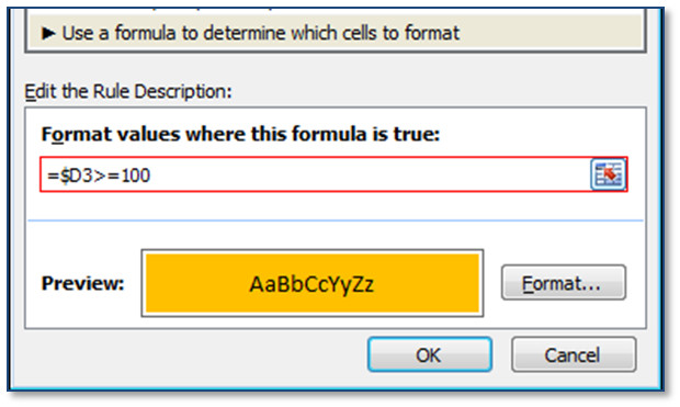
5. In the Edit the Rule Description section, click in the Format values where this formula is true, field, then type or select the first criteria value, the donation in cell D3, followed by the criteria, ‘>=100’ (no quotes).
   Note if using your mouse to select the cell, Excel will add ‘$’ to indicate absolute references. It is important that you remove the absolute reference indicator before the row number.
6. Click the Format button. The Format Cells dialog appears.
7. Click Fill tab, and select a Background Color.
8. Click OK. The dialog should look like this:
   
   
9. Click OK.

A few more notes on Conditional formats.

• To edit or delete the conditional formats: On the Home tab, in the Styles group, click Conditional Formatting and select Manage Rules.
• You can create multiple rules and order how they should be applied.

Experiment: change some contributions in the spreadsheet and see how the conditional formatting reformats the row.

Cheers!
hɔuᴉnb

Comments and questions are always welcome!