Looking for an easy way to highlight a column that is not in a table? Use COLUMN SELECT
Note: This tip works equally well when editing an email in Outlook.
Looking for an easy way to highlight a column that is not in a table? Use COLUMN SELECT
Click to enlarge
Column Select
Click insertion point at begining of text
Press ALT as you CLICK + DRAG to end point.
Once selected the text can be formatted or deleted. The selection collapses after your executed command.
Be smooth: ALT+CLICK instruction brings up the Thesaurus*, so be don’t click quickly. Column Select (ALT + CLICK + DRAG) works best to when you use a smooth, paint-like motion (more like Pollock than Seurat)
*(a deadly neolithic creature hellbent on correcting ingesting your text and regurgitating its own).
Here’s another cool feature of Excel: Speak Cells on Enter.
This can prove valuable as a means to verify accurate data entry. The only setup required is to add a button to your Quick Action Toolbar (QAT).
To setup:
RIGHT + CLICK on the QAT and select Customize Quick Access Toolbar.
Set the Choose commands from drop-down to All commands, then scroll down and select Speak Cells on Enter.
Click Add, then OK.
The button now appears on your QAT. Click button to toggle the feature on or off.
When active, each time you enter in a cell, the cell contents will be read back to you. Unlike other reader programs this voice is clear and rather pleasant (take note Acrobat).
Now if only you could select the voice, I’d take something along the lines of a HAL 9000, or K.I.T.T. model.
Additional voice features of Excel include:
Speak Cells
Speak Cells – Stop Speaking Cells
Speak Cells by Columns
Speak Cells by Rows
Stop Listening to Voices in My Head*
*available only to select consumers. What, I am not one of them? I am so! You keep out of this.
Looking for an easy method to move a table row up?
Place cursor on the row.
Press ALT + SHIFT + Up Arrow.
Repeat as necessary until the cursor is elevated to desired position. As you probably guessed, pressing ALT + SHIFT + Down Arrow moves the selected row down.
This trick is not just limited to tables. It also works with:
Bulleted text
Numbered lists
Outline text
Non-numbered paragraphs
IQ points
Okay, admittedly that last one was just wishful thinking :).
*Tip applies to Word versions 2003, 2007, 2010, and 2013. This tip may be relevant in earlier Word versions, but to confirm this I would have to pull out my old PC from its resting spot, on a shelf, under a pair of acid-wash jeans, wedged between an un-seeded Chia Pet and my Commodore VIC 20.
Here’s a quick Office tip that applies to Word, Excel and PowerPoint.
The Mark as Final feature enables you to protect a document to discourage editing. This simple seal of protectioncan easily be removed by the reader, should it be determined editing is necessary.
Note, this option is not designed to prevent edits, only to ward against unintentional editing. To render the document un-editable use other alternatives (for example, saving the file password protected or distributing a PDF version of the file).
To Apply Mark as Final
On the File tab, scroll down to Info, click Protect and select Mark as Final. A dialog will appear indicating “the file will be marked as final and saved.”
Click OK to confirm.
When backstage view is active, a notice appears in the status bar, indicating, “An author has marked this … as final to discourage editing.” The Application title bar also indicates that the file is Read-only. Reading, printing, and viewing options continue to function, but all editing features are disabled.
To remove the Mark as Final setting and restore edit functions repeat step 1, above. Alternatively, you can click the Edit Anyway button displayed on the info bar in the backstage view .
Here’s a quick tip that highlights PowerPoint’s easy to use Photo Album.
Remember the time when slideshow, meant a carousel of slides with you sitting in a dark room while [insert familial relation here] clicked through a series of pictures from some vacation?
No? Hmm, I may be dating myself. 😦
Take a retro moment; throw-away that text based presentation you have been struggling with (let’s face it, no one reads that stuff anyway) in favor of an old fashioned picture slideshow.
Create a Photo Album Slideshow:
On the Insert tab, in the Images group, click the top split of the Photo Album button. The Photo Album dialog appears.
Click the File/Disk button. The Insert New Pictures dialog appears.
Navigate to the folder that contains the pictures to be included and select those images. Note use CTRL + CLICK to ‘cherry pick’ images, or CLICK on the first picture and SHIFT + CLICK on the last to select that set of pictures.
Click OK to return the Photo Album dialog.
Optionally, adjust a picture’s settings by selecting that picture and then clicking the appropriate Move, Contrast or Rotate option.
Select a Picture layout (e.g., Fit to slide, 2 Pictures, etc.) and select a Theme.
Click Create.
Voila! Press F5 (shortcut) to run the slideshow
Should you need to edit the Photo album, click the bottom split of the Photo Album button and select Edit Photo Album.
Conditional Formatting makes it easy to visually highlight cells, based upon conditions (criteria) that you set. The conditional formats are dynamic, so as the data is edited, the criteria is tested, and the formats reapplied.
In a prior post, I mentioned how you can format an entire row or record based upon criteria found in one of that row’s fields. Here’s the step by step example, using the Charity Guest List data, used in the prior post.
Let’s demonstrate the COUNTIF using the first scenario. Count the number of guests who have donated more than $100
Rows conditionally formatted gold where donation is greater than or equal to $100
The intent is to format gold, those rows where the value in column D is $100 or greater.
A copy of this spreadsheet can be found here, on Google Drive. The file will open in a browser window/tab, in view mode. Click CTRL + S (PC) or select FILE, SAVE AS to download the file.
Open the file in Excel.
Select the donation data, cells A3:D15.
On the Home tab, in the Styles group, click the Conditional Formatting drop-down and select New Rule. The New Formatting Rule dialog will appear.
Select Use a formula to determine which cells to format.
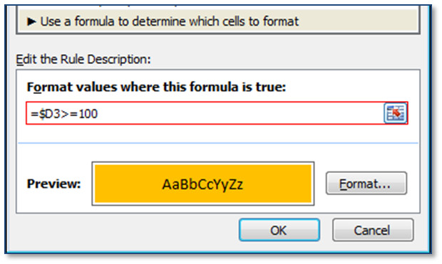
In the Edit the Rule Description section, click in the Format values where this formula is true, field, then type or select the first criteria value, the donation in cell D3, followed by the criteria, ‘>=100’ (no quotes). Note if using your mouse to select the cell, Excel will add ‘$’ to indicate absolute references. It is important that you remove the absolute reference indicator before the row number.
Click the Format button. The Format Cells dialog appears.
Click Fill tab, and select a Background Color.
Click OK. The dialog should look like this:
Click OK.
A few more notes on Conditional formats.
To edit or delete the conditional formats: On the Home tab, in the Styles group, click Conditional Formatting and select Manage Rules.
You can create multiple rules and order how they should be applied.
Experiment: change some contributions in the spreadsheet and see how the conditional formatting reformats the row.