Using DSUM

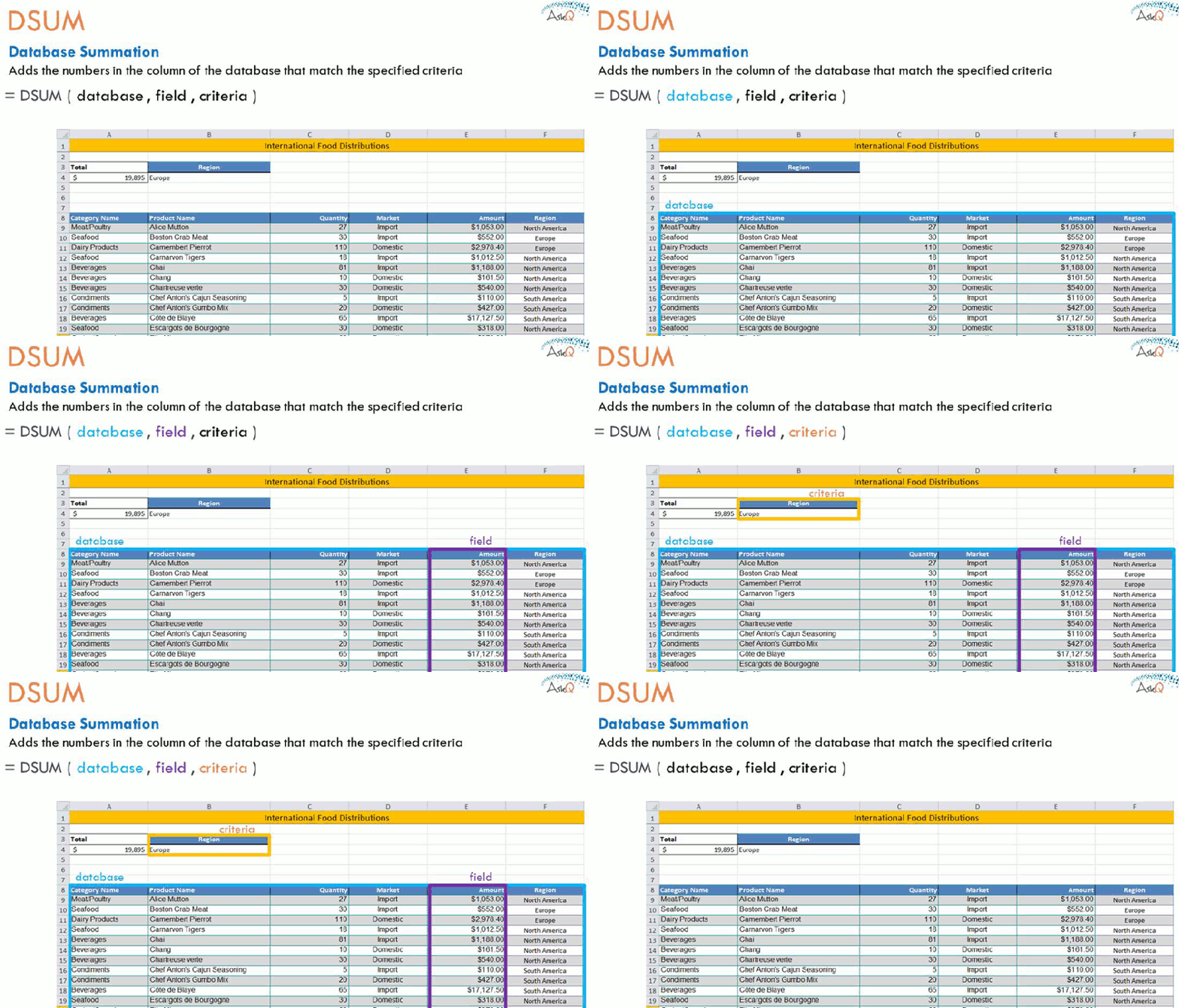
3 of 4: Summing values using DSUM

(revised and expanded from an earlier post)
In the previous posts we added Check Boxes to our spreadsheet and linked those Check Boxes to cells to display True when checked and False when unchecked. In this post, we take a brief break from Check Boxes to explore the DSUM function. But don't fret, in upcoming post we will tie Check Boxes and DSUM together to produce an interactive report.

DSUM, short for Database Summation, enables you to summarize data in a table (aka, database) based upon a specific condition (aka, criteria). Similar to the SUMIF function, DSUM can employ Boolean (i.e., AND/OR) logic in its criteria.

=DSUM( database, field, criteria)

• Database: the entire table, including row values, and headings
• Field: the column containing numbers to sum
• Criteria: condition to test for inclusion in the summary (contains field headings and value)

In the example depicted above, we sum the values in the Amount column based upon the criteria entered in B3:B4 (i.e., Region: Europe)

Watch this ~3m video to learn more.

 

Tip: when working with large data, name the cells to simplify formula entry.

To Name a Group of Cells

1. Select all the cells.
   Tip: select one cell, then press CTRL + A to select all contiguous (touching) cells
2. Click in the Name box, type name (e.g., “FoodInventory”) and press Enter.
   Note: Names cannot begin with a number, or include spaces.

Creating the Summation using DSUM

1. Type criteria, entering the field names on one row and the condition to test right below it
   (i.e., In B3 enter Region and in B4 enter Europe).
2. Select the cell to contain summation (i.e., A4).
3. On the Formulas tab, in the Function Library group, click Insert Function. The Insert Function dialog appears.
4. In the Search for function area, type DSUM and click Go. DSUM appears in the Selection function area.
5. Click OK. The Function Arguments dialog appears.
6. In the Database area type the name of database (i.e., FoodInventory).
   Tip: press F3 key to display list of named cells and select  from that list.
7. In the Field area type the column heading to summarize, in quotes (i.e., “Amount”).
   Alternatively, you can enter the number of the summation column, counting from left of the table (i.e., 5).
8. In the Criteria area, type or select the cells that contain the criteria; this includes the column heading(s) and value to search for (i.e., B3:B4).
9. Press OK.

Next and  Final: Automating the spreadsheet using DSUM and Check Boxes.

Cheers!

hɔuᴉnb

 
Previous post and additional reading:

• Adding Check Boxes
• Linking the Check Box to a Cell
• Formatting Indents in  Excel
• More Excel Tips

Comments and questions are always welcome!