Tag: AskQ

4 of 4: Automating the Spreadsheet using Check Boxes , If Statements, and DSUM

In the previous posts we added Check Boxes to our spreadsheet, linked Check Boxes to cells, and created a conditional summation using DSUM. In this post, we put this altogether with an interactive report. Using Check Boxes, IF statements, and DSUM, the user will select what criteria to sum by.

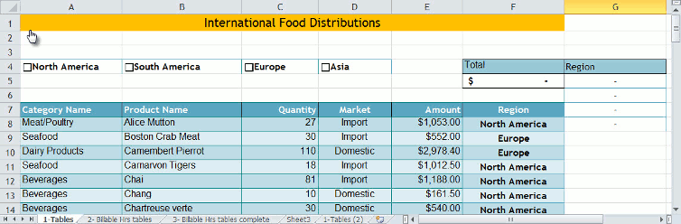
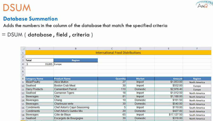
In the example depicted above, we sum the values in the Amount column based upon the criteria entered in column G.

Watch this ~3m video to learn more.

 

Adding and Linking the Check Boxes

1. Insert two blank rows above the database.
2. In the second blank row, add Check Box Form controls for each criteria value to be included in the summary. In the example depicted, we created Check Boxes for each region (see Adding a Check Box for instructions).
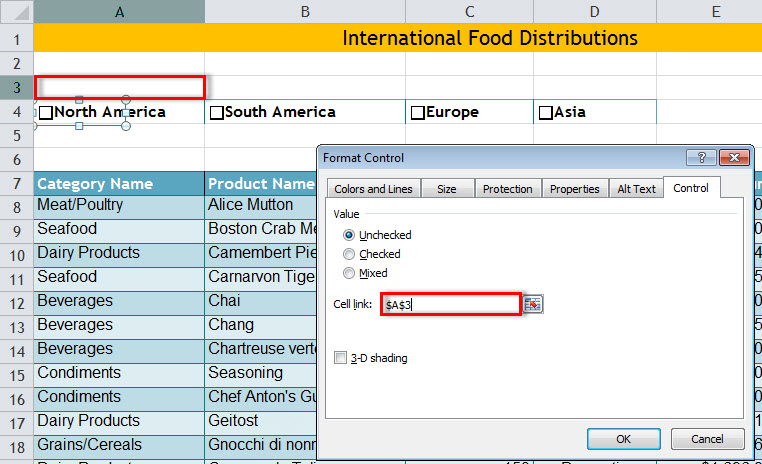
3. Link the Check Box to the cell above: Right + Click on the Check Box, select Format Control, and enter above cell in the Cell link field (for more detailed instructions click here ). Repeat for each Check Box.

 

Creating the Criteria Column

We will use the IF function to copy the Checked labels into the criteria range

1. In a blank column, enter the field name into the cell (i.e., ‘Region’) .
2. Move cursor to the cell immediately below.
3. On the Formula tab, in the Function Library group, click Logical and select IF.
4. In the  Logical_test field, select or type Linked cell above the Check Box. In the example depicted below enter A3 to test Checked state for ‘North America.’
5. In the Value_if_true field, select or type the Check Box cell. In the example depicted below enter A4 for the text ‘North America.’
6. In the Value_if_false field, type ” – ” (dash in quotes).
7. Click OK.

Repeat steps 2 through 7 for each Check Box value to be included in the summation.

To  test the IF statements, check and uncheck the boxes. When checked, the text associated with that Check Box will appear in the criteria column.

 

Inserting the DSUM function

1. Select the cell to contain summation (i.e., F5).
2. On the Formulas tab, in the Function Library group, click Insert Function. The Insert Function dialog appears.
3. In the Search for function area, type DSUM and click Go. DSUM appears in the Selection function area.
4. Click OK. The Function Arguments dialog appears.
5. In the Database area, enter either the saved name or cell reference for the table (e.g., FoodInventory or A7:F255).
6. In the Field area type the column heading to summarize, in quotes (i.e., “Amount”).
7. In the Criteria area, type or select the cells that contain the criteria; this includes the column heading(s) and value to search for (i.e., G4:G8).
8. Press OK.

Tip: Hide the criteria column to make the report appear less cluttered.

That’s it. Now, to add a region to the summation, check that region’s Check Box. To remove a region from the summation, uncheck it.

 

Cheers!

hɔuᴉnb

 

Previous post and additional reading:

• Using DSUM
• Adding Check Boxes
• Linking the Check Box to a Cell
• Formatting Indents in  Excel
• More Excel Tips

Comments and questions are always welcome!

3 of 4: Summing values using DSUM

(revised and expanded from an earlier post)
In the previous posts we added Check Boxes to our spreadsheet and linked those Check Boxes to cells to display True when checked and False when unchecked. In this post, we take a brief break from Check Boxes to explore the DSUM function. But don't fret, in upcoming post we will tie Check Boxes and DSUM together to produce an interactive report.

DSUM, short for Database Summation, enables you to summarize data in a table (aka, database) based upon a specific condition (aka, criteria). Similar to the SUMIF function, DSUM can employ Boolean (i.e., AND/OR) logic in its criteria.

=DSUM( database, field, criteria)

• Database: the entire table, including row values, and headings
• Field: the column containing numbers to sum
• Criteria: condition to test for inclusion in the summary (contains field headings and value)

In the example depicted above, we sum the values in the Amount column based upon the criteria entered in B3:B4 (i.e., Region: Europe)

Watch this ~3m video to learn more.

 

Tip: when working with large data, name the cells to simplify formula entry.

To Name a Group of Cells

1. Select all the cells.
   Tip: select one cell, then press CTRL + A to select all contiguous (touching) cells
2. Click in the Name box, type name (e.g., “FoodInventory”) and press Enter.
   Note: Names cannot begin with a number, or include spaces.

Creating the Summation using DSUM

1. Type criteria, entering the field names on one row and the condition to test right below it
   (i.e., In B3 enter Region and in B4 enter Europe).
2. Select the cell to contain summation (i.e., A4).
3. On the Formulas tab, in the Function Library group, click Insert Function. The Insert Function dialog appears.
4. In the Search for function area, type DSUM and click Go. DSUM appears in the Selection function area.
5. Click OK. The Function Arguments dialog appears.
6. In the Database area type the name of database (i.e., FoodInventory).
   Tip: press F3 key to display list of named cells and select  from that list.
7. In the Field area type the column heading to summarize, in quotes (i.e., “Amount”).
   Alternatively, you can enter the number of the summation column, counting from left of the table (i.e., 5).
8. In the Criteria area, type or select the cells that contain the criteria; this includes the column heading(s) and value to search for (i.e., B3:B4).
9. Press OK.

Next and  Final: Automating the spreadsheet using DSUM and Check Boxes.

Cheers!

hɔuᴉnb

 
Previous post and additional reading:

• Adding Check Boxes
• Linking the Check Box to a Cell
• Formatting Indents in  Excel
• More Excel Tips

Comments and questions are always welcome!

1 of 4: Adding Check Boxes

In these four post we will will create an interactive report using Check boxes and DSUM (and without the using macros). In this first of four, we start with adding Check Boxes.

Since Excel 2007, the use of macros in spreadsheets have added an additional element of complexity. Macros must now be stored in XLSM format, which raises a red flag in excel as a potential threat. In this series of posts, we eschew VBA and ActiveX automation, in exchange for ‘old fashioned’ excel programming, using form controls and statistical functions.

Adding Check boxes to your spreadsheet can make it easier for you and your reviewers to edit spreadsheet data. The Check box tool is found on the Developer Tab. To add the Developer tab, click File, Options, Customize Ribbon, and check Developer.

To Add a Check box

1. On the Developer tab, in the Controls group, click Insert Check box (Form Control).
2. Using the mouse, Click & Drag to draw a Check box control. A Check box control is placed, consisting of the Check box and the label text.
   Tip: Hold down the ALT key as you Click & Drag to draw an object equal in size to the selected cell.
3. Right + Click on the Check box control and select Edit Text. An insertion point appears.
4. Delete the Check box label text (e.g. Check Box 1).
5. Click & Drag rightmost selection handle to reduce the size of the Check box control.
6. Enter your text into the cell that contains the Check box.
   Tip: To indent the text, on the Home ribbon, click the Alignment dialog launcher and increase the cell Indent to 2.

 

Next: Linking the Check Box to a Cell!

Cheers!

hɔuᴉnb

Additional reading:

• Formatting Indents in  Excel
• Excel Data Consolidation
• More Excel Tips

Comments and questions are always welcome!