Linking the Check Box to a Cell

2 of 4: Linking the Check Box to a Cell

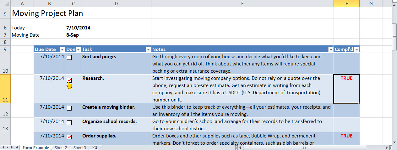
In the earlier post, Adding Check Boxes, we added the Form Check Box control to our spreadsheet. In this post we explore adding an ActiveX Check Box to the spreadsheet, and how to link a Check Box to a cell. The linked cell will display True, when the Check Box is checked, and False when unchecked.
Click to enlarge
Form Check Box with Linked Cell


Form Check Box

Of the two types of Check Box controls, Form and ActiveX, the Form control is the simpler of the two types.

Form Check Box features:

  • simple management, with comparatively few options
  • compatible with the XLS file format (Excel 2003 and earlier)

Watch this ~3m video to see how to place the Form Check Box and link it to a cell.

To Link the Check Box Form Control to a Cell

  1. Add the Form Check Box control (for details, see earlier post or review the above video).
  2. Right + Click on the Check Box control and select Format Control.  The Format Control dialog appears.
  3. On the Control tab, click in the Cell link field, then type or select the cell.
  4. OK.

ActiveX Check Box

For more programming power, use the ActiveX Check Box. Similar to Form Check Boxes, the ActiveX Check Box has additional options.

ActiveX Check Box features:

  • additional formatting and programming options
  • designed to be associated with macros
  • compatible with the XLSM and XLTM file formats (macro enabled file and macro enabled template, respectively)

Watch this ~3m video to see how to place the ActiveX Check Box and link it to a cell.

To Link the Check Box ActiveX Control to a Cell

  1. On the Developer Tab, In the Control group, Click the ActiveX Check Box control, then Click + Drag to place on spreadsheet.
    Note: the spreadsheet is automatically placed in Design Mode.
  2. Right + Click on the Check Box control and select Properties.  The Properties dialog appears.
  3. Click in the Caption property field and delete the text (i.e., CheckBox1).
  4. For the BackStyle property, click drop-down and select 0 – fmBackStyleTransparent.
  5. Click in the LinkedCell property field and type the cell reference (i.e. F10).
  6. Close the Property dialog.
  7. On the Developer tab, click Design Mode to toggle Design Mode off.


Next: Using DSUM!

Cheers!

hɔuᴉnb

Previous post and additional reading:

Comments and questions are always welcome!

Adding Check Boxes

1 of 4: Adding Check Boxes

In these four post we will will create an interactive report using Check boxes and DSUM (and without the using macros). In this first of four, we start with adding Check Boxes.

Since Excel 2007, the use of macros in spreadsheets have added an additional element of complexity. Macros must now be stored in XLSM format, which raises a red flag in excel as a potential threat. In this series of posts, we eschew VBA and ActiveX automation, in exchange for ‘old fashioned’ excel programming, using form controls and statistical functions.

Check Box

Adding Check boxes to your spreadsheet can make it easier for you and your reviewers to edit spreadsheet data. The Check box tool is found on the Developer Tab. To add the Developer tab, click File, Options, Customize Ribbon, and check Developer.

To Add a Check box

  1. On the Developer tab, in the Controls group, click Insert Check box (Form Control).
  2. Using the mouse, Click & Drag to draw a Check box control. A Check box control is placed, consisting of the Check box and the label text.
    Tip: Hold down the ALT key as you Click & Drag to draw an object equal in size to the selected cell.
  3. Right + Click on the Check box control and select Edit Text. An insertion point appears.
  4. Delete the Check box label text (e.g. Check Box 1).
  5. Click & Drag rightmost selection handle to reduce the size of the Check box control.
  6. Enter your text into the cell that contains the Check box.
    Tip: To indent the text, on the Home ribbon, click the Alignment dialog launcher and increase the cell Indent to 2.


alignmentNext: Linking the Check Box to a Cell!

Cheers!

hɔuᴉnb

Additional reading:

Comments and questions are always welcome!

April Fools’ Tips & Tricks

 Happy April 1st.

First the tip: When leaving your PC unattended, press WINDOWS KEY + L to lock your screen and keyboard. This will prevent you from falling prey to any seasonal pranks (like these).

Now the tricksHere is a short list of relatively harmless April Fools’ pranks you could play on a friend’s unlocked PC.

Windows

Change the Double+Click speed

“My mouse is broken”

  1. Click Start, type “mouse”, select Settings filter, then click Change Mouse Settings.
  2. Select the Buttons Tab.
  3. In the Double-Click area move the slider bar to the fastest setting.
  4. Click OK.

Flip the Screen

They might need to stand on their heads for a bit

  • Press CTRL + ALT + DOWN ARROW to rotate the display 180°
  • To return screen to normal press CTRL + ALT + UP ARROW

Excel

Cursor Up on Enter

Gravity will seem to have taken a holiday as Enter moves the cursor up instead of down.

  1. File/ Options / Advanced.
  2. In the Editing section, check After Pressing Enter move selection,
  3. For Direction select Up.
  4. Ok.

Ribbonus-Interruptus

Formula entry is problematic when pressing = moves the focus from the sheet to the Ribbon.

  1. File/ Options / Advanced.
  2. In the Lotus Compatibility section, in the Microsoft menu key field type  =.
  3. Ok.


Cheers!

hɔuᴉnb

MS Office on the iPad

Microsoft Office, for the iPad is finally here!

After years of working with 3rd party viewers, you can now open and view Documents, Spreadsheets and Slides using MS Office for iPad. Tap the Share button to open an attachment in its respective Office application. The look and feel are just like using a streamlined (portable) version of your desktop Office.  That is to say, it won’t have all the same features, but for on-the-go computing it works great.

The apps are free, however, to unlock the full potential you’ll need to subscribe to Office 365. This is the Office via Cloud (aka SAS) and will enable you to create, save and edit files.

I have never been a big fan of editing on a tablet and Word for the iPad has yet to convince me otherwise. I do, however, appreciate being able to view and create spreadsheets while away from my desktop, using Excel for the iPad. But the real winner thus far (less than 24 hours into install) is PowerPoint for the iPad. Now I can display a presentation directly from my iPad to a projector/monitor and use familiar presentation controls, complete with laser pen, highlighter and notes (sweet!)

Comments and questions are always welcome!hɔuᴉnb


Excel NCAA templates

March Madness is upon us!

In 1892 Coach James Naismith hammered two peach baskets into the gym balcony, and forever changed how we use Excel!

NCAA_LooneyToons

Using these free templates available in Excel, you can plot out your final four projections!

To access NCAA templates

  1. Click File and select New.
  2. In the Search Office Templates field type ‘NCAA‘ (no quotes) and press the search arrow. The search results will populate the dialog.
  3. Select preferred template and click Download.

ncaa

from Wikipedia:

[Naismith] divided his class of 18 into 2 teams of 9 players each and set about to teach them the basics of his new game of Basketball. The objective of the game was to throw the [ball], into the fruit baskets nailed to the lower railing of the gym balcony. Every time a point was scored, the game was halted so the janitor could bring out a ladder and retrieve the ball. Later, the bottoms of the fruit baskets were removed. The first public basketball game was played in Springfield, MA, on March 11, 1892. That day, he asked his class to play a match in the Armory Street court: 9 versus 9, using a soccer ball and two peach baskets.

Cheers!

hɔuᴉnb

Additional reading:

Comments and questions are always welcome!

Excel Indents

Excel Indents

Want to make your spreadsheet more legible? Indents, added where appropriate, will make your spreadsheet easier to mentally digest.
Sadly, it won’t make bad financial news easier to swallow.

Watch this 15 second video to learn the what you need to know.

Indent a cell

  1. Select the cell(s) to indent
  2. On the Home tab, in the Alignment Group, click the dialog launcher Dialog Launcher
    (or press CTRL + SHIFT + F to display the Font dialog and click the Alignment tab).
  3. In the Text alignment section, click the Horizontal drop-down and select Left (Indent).
  4. In the Indent field, type or select preferred indent increment (i.e., 1, 2).
  5. Click OK.

Cheers!

hɔuᴉnb

Additional reading:

Comments and questions are always welcome!

Excel Sparklines

Be Trendy!

Sparklines

Sparklines are an easy way to add visual trend-lines to your tabular data.
And what better way to distract your audience than by dangling something sparkly in front of them!

Watch this 60 second video to learn the what you need to know.

Inserting Sparklines to your Excel data

  1. On the Insert tab, in the Sparklines group, click Sparkline type (e.g., Line). The Create Sparklines dialog appears.
  2. In the Data Range field enter the values to be charted.
  3. In the Location Range field enter cell range where char is to be displayed.
  4. Click OK.

Tip: With an inserted sparkline selected, the Sparklines Tools: Design tab appears on the Ribbon. Use the tools on this tab to change colors and add markers.

Cheers!

hɔuᴉnb

Additional reading:

Comments and questions are always welcome!