Linking the worksheet name to a cell in the spreadsheet is easily accomplished using Excel’s CELL function. Once joined by the MID and SEARCH functions, you need only change the sheet’s name and the linked cell will update to match.
Click to view at full resolution
Displaying the Sheet Name in a Cell
Type (or copy and paste) the following formula into a cell
During the next series of posts I will demonstrate some commonly used Text functions. In the illustrated example we populate a CustomerCode column by combining
the first letter of the first name,
the first 4 letters of the last name, and
the last 4 digits of the phone number
=LEFT
Returns the leftmost character(s) of a cell, as specified by the optional Num_chars argument.
click image to view at full resolution
Using the LEFT function to copy the leftmost characters of a cell
Select cell to display the result.
On the Formulas tab, in the Function Library group, click Text drop-down and select LEFT.
In Text field select or type cell containing text.
In the Num_chars field enter the number of characters to copy. When left blank the result is only the leftmost character.
Click OK.
Concatenate using ‘&’
Use the Ampersand (&) to concatenate (combine) text. For example, with “North” in A1 and “West” in B1, the formula =A1&B1 returns “NorthWest”
=RIGHT
Returns the rightmost character(s) of a cell, as specified by the optional Num_chars argument.
Using the RIGHT function to copy rightmost character(s) of a cell
Select cell to display the result.
On the Formulas tab, in the Function Library group, click Text drop-down and select RIGHT.
In Text field select or type cell containing text.
In the Num_chars field enter number of characters to copy. When left blank the result is only the rightmost character.
After completing the J.P. Morgan Corporate Challenge 5K race I was curious: how many other runners had a similar finish time as I? What an Excel-lent opportunity for a Histogram!
A Histogram analyzes values, groups those numbers into bins, (population frequencies) of your choosing, and displays that data in a table or chart. The Histogram tool is part of the Data Analysis Toolpak. It may not initially appear on your ribbon, but is a cinch to install.
Adding the Data Analysis Toolpak
On the Ribbon, click File, then Options.
Click Add-ins.
On the Manage drop-down, select Excel Add-ins and click Go.
Select Analysis Toolpak and click OK.
For a simple Histogram, here’s what you will need:
Input Range: cells containing values to be reviewed. The range must be sorted in ascending sequence.
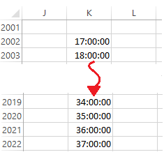
Bin Range: cells to act as virtual bins within which Excel will place matching numbers. For example, a teacher grading a test might use Bin values for the test scores she wants to lump together. Bin range is an optional; if left blank, Excel will create Bins.In my example (below) the Bin values are increments of one minute, between 17 and 37 minutes (the fastest and longest finishing times).
Bin range, using finish times from 17:00 to 37:00
Output: Location for the Histogram table. These options include Range, New Worksheet, and New Workbook.
Chart Output: (optional) charts the Histogram table output.
Creating the Histogram Table and Chart
On Data tab of the Ribbon, click Data Analysis. The Data Analysis dialog appears.
Select Histogram and click OK. The Histogram dialog appears.
Select or enter the Input Range (e.g., E11:E2804) , Bin Range (e.g., K13:K32), and Output range (e.g. M12).,
Creating Defined Names enables you to take advantage of a host of excel features and shortcuts. This post shows one easy method to create Defined Names from your selection and showcases a nifty method to find where two Defined names intersect.
This tip involves naming cells, also known as Defined Names. Among the many benefits, Defined Names can be used to:
quickly navigate large spreadsheets
easily define print areas
simplify formula entry
In the below table you want to easily reference the data in any given column or row. Since the data is in a table you can easily create a Defined Name, for each column and row, using the Create from Selection command.
Creating Defined Names From Selection
Select all the cells in the table. Tip: select one cell, then press CTRL + A.
On the Formulas tab, in the Defined Names group, click Create from Selection. The Create Names from Selection dialog appears.
Check Top row and Left column.
OK.
To display the Defined Names, press F3 or click the Name Box drop-down. Defined Names will also appear as you enter formulas, preceded by the name tag icon.
PowerTip: The intersection of two Defined Names can be displayed using a formula.
Using Defined Names to Display the Intersecting Value
In this post, we put this altogether with an interactive report. Using check boxes and DSUM the user will select what criteria to sum by.
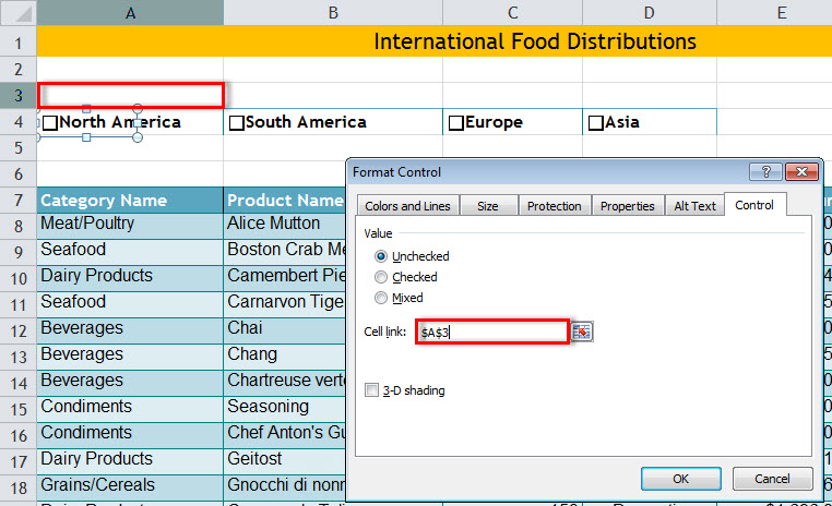
4 of 4: Automating the Spreadsheet using Check Boxes , If Statements, and DSUM
In the previous posts we added Check Boxes to our spreadsheet, linked Check Boxes to cells, and created a conditional summation using DSUM. In this post, we put this altogether with an interactive report. Using Check Boxes, IF statements, and DSUM, the user will select what criteria to sum by.
Click to enlarge
In the example depicted above, we sum the values in the Amount column based upon the criteria entered in column G.
Watch this ~3m video to learn more.
Adding and Linking the Check Boxes
Insert two blank rows above the database.
In the second blank row, add Check Box Form controls for each criteria value to be included in the summary. In the example depicted, we created Check Boxes for each region (see Adding a Check Box for instructions).
Link the Check Box to the cell above: Right + Click on the Check Box, select Format Control, and enter above cell in the Cell link field (for more detailed instructions click here ). Repeat for each Check Box.
Creating the Criteria Column
We will use the IF function to copy the Checked labels into the criteria range
In a blank column, enter the field name into the cell (i.e., ‘Region’) .
Move cursor to the cell immediately below.
On the Formula tab, in the Function Library group, click Logical and select IF.
In the Logical_test field, select or type Linked cell above the Check Box. In the example depicted below enter A3 to test Checked state for ‘North America.’
In the Value_if_true field, select or type the Check Box cell. In the example depicted below enter A4 for the text ‘North America.’
In the Value_if_false field, type ” – ” (dash in quotes).
Click OK.
Repeat steps 2 through 7 for each Check Box value to be included in the summation.
To test the IF statements, check and uncheck the boxes. When checked, the text associated with that Check Box will appear in the criteria column.
Inserting the DSUM function
Select the cell to contain summation (i.e., F5).
On the Formulas tab, in the Function Library group, click Insert Function. The Insert Function dialog appears.
In the Search for function area, type DSUM and click Go. DSUM appears in the Selection function area.
Click OK. The Function Arguments dialog appears.
In the Database area, enter either the saved name or cell reference for the table (e.g., FoodInventory or A7:F255).
In the Field area type the column heading to summarize, in quotes (i.e., “Amount”).
In the Criteria area, type or select the cells that contain the criteria; this includes the column heading(s) and value to search for (i.e., G4:G8).
Press OK.
Tip:Hide the criteria column to make the report appear less cluttered.
That’s it. Now, to add a region to the summation, check that region’s Check Box. To remove a region from the summation, uncheck it.
(revised and expanded from an earlier post)
In the previous posts we added Check Boxes to our spreadsheet and linked those Check Boxes to cells to display True when checked and False when unchecked. In this post, we take a brief break from Check Boxes to explore the DSUM function. But don't fret, in upcoming post we will tie Check Boxes and DSUM together to produce an interactive report.
Click to enlarge
DSUM, short for Database Summation, enables you to summarize data in a table (aka, database) based upon a specific condition (aka, criteria). Similar to the SUMIF function, DSUM can employ Boolean (i.e., AND/OR) logic in its criteria.
=DSUM( database, field, criteria)
Database: the entire table, including row values, and headings
Field: the column containing numbers to sum
Criteria: condition to test for inclusion in the summary (contains field headings and value)
In the example depicted above, we sum the values in the Amount column based upon the criteria entered in B3:B4 (i.e., Region: Europe)
Watch this ~3m video to learn more.
Tip: when working with large data, name the cells to simplify formula entry.
To Name a Group of Cells
Select all the cells. Tip: select one cell, then press CTRL + A to select all contiguous (touching) cells
Click in the Name box, type name (e.g., “FoodInventory”) and press Enter. Note: Names cannot begin with a number, or include spaces.
Creating the Summation using DSUM
Type criteria, entering the field names on one row and the condition to test right below it
(i.e., In B3 enter Region and in B4 enter Europe).
Select the cell to contain summation (i.e., A4).
On the Formulas tab, in the Function Library group, click Insert Function. The Insert Function dialog appears.
In the Search for function area, type DSUM and click Go. DSUM appears in the Selection function area.
Click OK. The Function Arguments dialog appears.
In the Database area type the name of database (i.e., FoodInventory). Tip: press F3 key to display list of named cells and select from that list.
In the Field area type the column heading to summarize, in quotes (i.e., “Amount”).
Alternatively, you can enter the number of the summation column, counting from left of the table (i.e., 5).
In the Criteria area, type or select the cells that contain the criteria; this includes the column heading(s) and value to search for (i.e., B3:B4).
Press OK.
Next and Final: Automating the spreadsheet using DSUM and Check Boxes.


 .
.