Looking for an easy way to highlight a column that is not in a table? Use COLUMN SELECT
Note: This tip works equally well when editing an email in Outlook.
Looking for an easy way to highlight a column that is not in a table? Use COLUMN SELECT
Click to enlarge
Column Select
Click insertion point at begining of text
Press ALT as you CLICK + DRAG to end point.
Once selected the text can be formatted or deleted. The selection collapses after your executed command.
Be smooth: ALT+CLICK instruction brings up the Thesaurus*, so be don’t click quickly. Column Select (ALT + CLICK + DRAG) works best to when you use a smooth, paint-like motion (more like Pollock than Seurat)
*(a deadly neolithic creature hellbent on correcting ingesting your text and regurgitating its own).
While Amazon’s drone plans stall, Silicon Valley startup, Matternet, is piloting (pun intended) a drone service in Bhutan. This aerobo (aerial-robotic) fleet is providing a means of delivering medicinal supplies to rural communities.
Negotiating meeting schedules between time zones can be tricky. Here are two simple methods to help keep track of time in other regions:
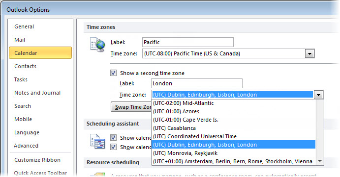
Add Additional Time Zone to the Outlook Calendar
In Outlook, click File, then select Options. The Outlook Options dialog appears.
At left, select Calendar, then scroll down to the Time zones section.
In the Label area type a brief description for the local time zone.
Check Show a second time zone.
In the second Label area, type a brief description for the second time zone.
Select additional time zonefrom the second Time zone drop down.
OK.
Outlook Calendar Options
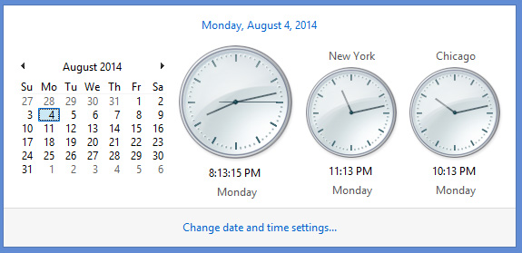
To Add Time zones to Windows Taskbar
The windows taskbar has the ability to show two additional time zones.
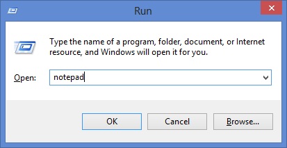
Windows 8 Time Display
RIGHT + CLICK on time displayed in lower right corner of taskbar.
Select Adjust date/time.
Click Additional Clocks tab.
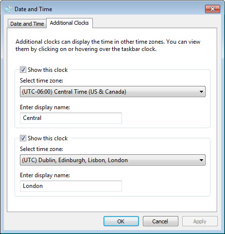
Check Show this clock.
For each additional time zone, check Show this clock, select time zone from the drop-down, then enter a name in the field below.
OK.
Additional Clocks dialog (CLICK to enlarge)
For additional multi-regional scheduling resources, visit the World Clock website. There you will find meeting calculators, daylight savings information and interactive maps.
In this post, we put this altogether with an interactive report. Using check boxes and DSUM the user will select what criteria to sum by.
4 of 4: Automating the Spreadsheet using Check Boxes , If Statements, and DSUM
In the previous posts we added Check Boxes to our spreadsheet, linked Check Boxes to cells, and created a conditional summation using DSUM. In this post, we put this altogether with an interactive report. Using Check Boxes, IF statements, and DSUM, the user will select what criteria to sum by.
Click to enlarge
In the example depicted above, we sum the values in the Amount column based upon the criteria entered in column G.
Watch this ~3m video to learn more.
Adding and Linking the Check Boxes
Insert two blank rows above the database.
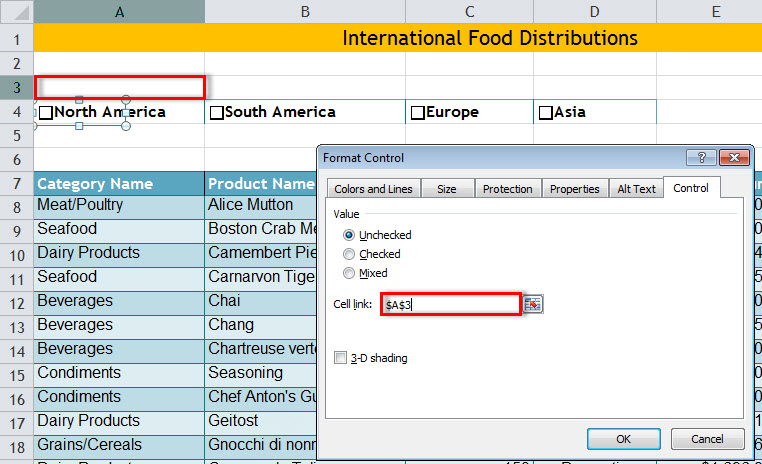
In the second blank row, add Check Box Form controls for each criteria value to be included in the summary. In the example depicted, we created Check Boxes for each region (see Adding a Check Box for instructions).
Link the Check Box to the cell above: Right + Click on the Check Box, select Format Control, and enter above cell in the Cell link field (for more detailed instructions click here ). Repeat for each Check Box.
Creating the Criteria Column
We will use the IF function to copy the Checked labels into the criteria range
In a blank column, enter the field name into the cell (i.e., ‘Region’) .
Move cursor to the cell immediately below.
On the Formula tab, in the Function Library group, click Logical and select IF.
In the Logical_test field, select or type Linked cell above the Check Box. In the example depicted below enter A3 to test Checked state for ‘North America.’
In the Value_if_true field, select or type the Check Box cell. In the example depicted below enter A4 for the text ‘North America.’
In the Value_if_false field, type ” – ” (dash in quotes).
Click OK.
Repeat steps 2 through 7 for each Check Box value to be included in the summation.
To test the IF statements, check and uncheck the boxes. When checked, the text associated with that Check Box will appear in the criteria column.
Inserting the DSUM function
Select the cell to contain summation (i.e., F5).
On the Formulas tab, in the Function Library group, click Insert Function. The Insert Function dialog appears.
In the Search for function area, type DSUM and click Go. DSUM appears in the Selection function area.
Click OK. The Function Arguments dialog appears.
In the Database area, enter either the saved name or cell reference for the table (e.g., FoodInventory or A7:F255).
In the Field area type the column heading to summarize, in quotes (i.e., “Amount”).
In the Criteria area, type or select the cells that contain the criteria; this includes the column heading(s) and value to search for (i.e., G4:G8).
Press OK.
Tip:Hide the criteria column to make the report appear less cluttered.
That’s it. Now, to add a region to the summation, check that region’s Check Box. To remove a region from the summation, uncheck it.
(revised and expanded from an earlier post)
In the previous posts we added Check Boxes to our spreadsheet and linked those Check Boxes to cells to display True when checked and False when unchecked. In this post, we take a brief break from Check Boxes to explore the DSUM function. But don't fret, in upcoming post we will tie Check Boxes and DSUM together to produce an interactive report.
Click to enlarge
DSUM, short for Database Summation, enables you to summarize data in a table (aka, database) based upon a specific condition (aka, criteria). Similar to the SUMIF function, DSUM can employ Boolean (i.e., AND/OR) logic in its criteria.
=DSUM( database, field, criteria)
Database: the entire table, including row values, and headings
Field: the column containing numbers to sum
Criteria: condition to test for inclusion in the summary (contains field headings and value)
In the example depicted above, we sum the values in the Amount column based upon the criteria entered in B3:B4 (i.e., Region: Europe)
Watch this ~3m video to learn more.
Tip: when working with large data, name the cells to simplify formula entry.
To Name a Group of Cells
Select all the cells. Tip: select one cell, then press CTRL + A to select all contiguous (touching) cells
Click in the Name box, type name (e.g., “FoodInventory”) and press Enter. Note: Names cannot begin with a number, or include spaces.
Creating the Summation using DSUM
Type criteria, entering the field names on one row and the condition to test right below it
(i.e., In B3 enter Region and in B4 enter Europe).
Select the cell to contain summation (i.e., A4).
On the Formulas tab, in the Function Library group, click Insert Function. The Insert Function dialog appears.
In the Search for function area, type DSUM and click Go. DSUM appears in the Selection function area.
Click OK. The Function Arguments dialog appears.
In the Database area type the name of database (i.e., FoodInventory). Tip: press F3 key to display list of named cells and select from that list.
In the Field area type the column heading to summarize, in quotes (i.e., “Amount”).
Alternatively, you can enter the number of the summation column, counting from left of the table (i.e., 5).
In the Criteria area, type or select the cells that contain the criteria; this includes the column heading(s) and value to search for (i.e., B3:B4).
Press OK.
Next and Final: Automating the spreadsheet using DSUM and Check Boxes.
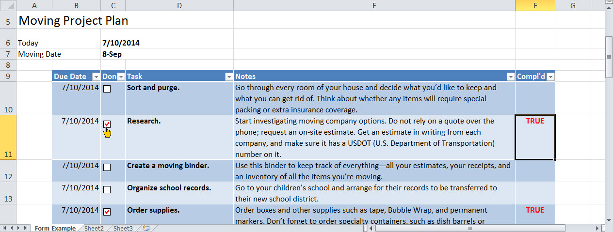
In the earlier post, Adding Check Boxes, we added the Form Check Box control to our spreadsheet. In this post we explore adding an ActiveX Check Box to the spreadsheet, and how to link a Check Box to a cell. The linked cell will display True, when the Check Box is checked, and False when unchecked.
Form Check Box with Linked Cell
Form Check Box
Of the two types of Check Box controls, Form and ActiveX, the Form control is the simpler of the two types.
Form Check Box features:
simple management, with comparatively few options
compatible with the XLS file format (Excel 2003 and earlier)
Watch this ~3m video to see how to place the Form Check Box and link it to a cell.
To Link the Check Box Form Control to a Cell
Add the Form Check Box control (for details, see earlier post or review the above video).
Right + Click on the Check Box control and select Format Control. The Format Control dialog appears.
On the Control tab, click in the Cell link field, then type or select the cell.
OK.
ActiveX Check Box
For more programming power, use the ActiveX Check Box. Similar to Form Check Boxes, the ActiveX Check Box has additional options.
ActiveX Check Box features:
additional formatting and programming options
designed to be associated with macros
compatible with the XLSM and XLTM file formats (macro enabled file and macro enabled template, respectively)
Watch this ~3m video to see how to place the ActiveX Check Box and link it to a cell.
To Link the Check Box ActiveX Control to a Cell
On the Developer Tab, In the Control group, Click the ActiveX Check Box control, then Click + Drag to place on spreadsheet. Note: the spreadsheet is automatically placed in Design Mode.
Right + Click on the Check Box control and select Properties. The Properties dialog appears.
Click in the Caption property field and delete the text (i.e., CheckBox1).
For the BackStyle property, click drop-down and select 0 – fmBackStyleTransparent.
Click in the LinkedCell property field and type the cell reference (i.e. F10).
Close the Property dialog.
On the Developer tab, click Design Mode to toggle Design Mode off.


