April is upcoming and I am handing out Easter Apples Eggs! iOS7 has been out for some months now, so this post may seem overdue. In defense, I was initially an un-fan of the new OS. Over time it has shown itself to be ‘a good thing’. So now, having made my peace with it, I am highlighting some of the better and under-exposed features.
My favorite of iOS7 features.
Spotlight Search
Swipe down from Home screen. Previously, you had to swipe all the way to the left most Home screen page. Now you can access Spotlight Search from any Home screen page. Use this to locate everything (i.e., apps, messages, contacts).
Control Center
Swipe up from bottom of the screen to access Control Center. From here you have access to key features (camera, airplane mode, music) without having to navigate to the Settings app.This feature can also be disabled if it interferes with a particular app’s swipe gesture. To manage settings, open the Settings app and tap Control Center.
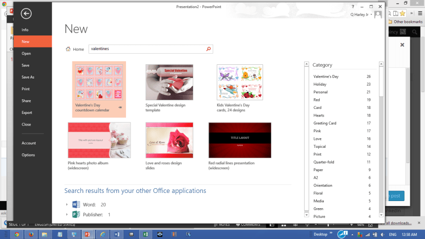
Flick to stop running apps
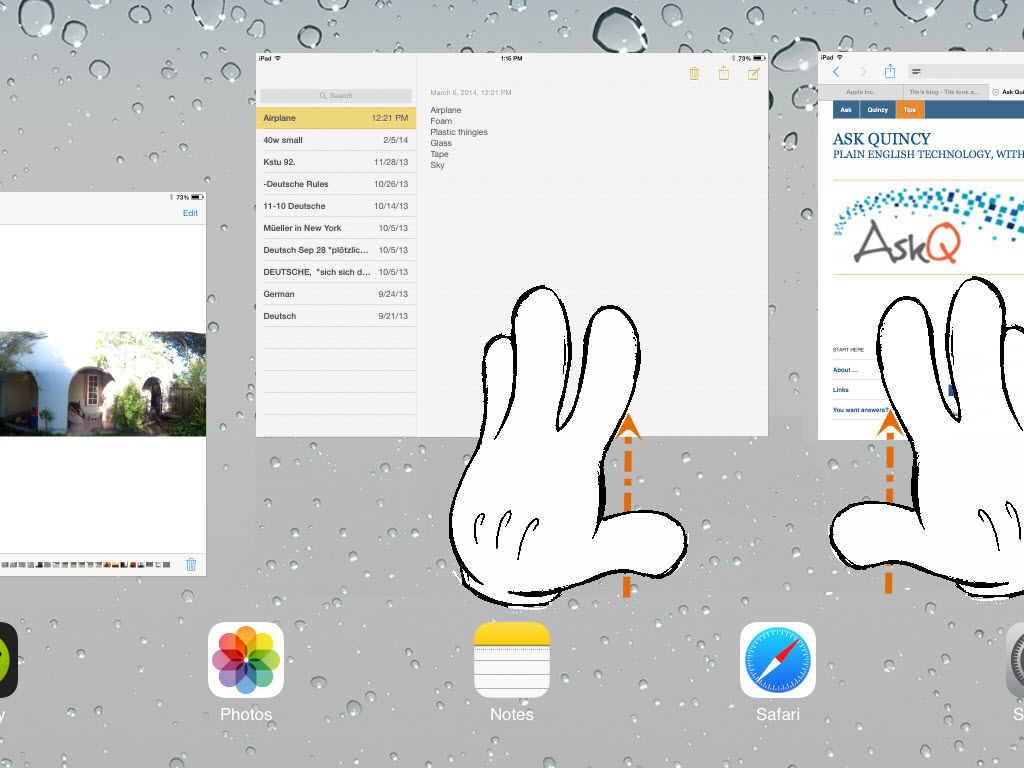
Double press the Home button to display running apps, then Flick app up& away to terminate. This gesture is far more satisfying than the previous ‘click the x‘ method.Bonus: you can flick-close multiple apps at a time!
Camera Burst Mode
From the Camera app, Press & Hold Capture button to take rapid fire shots. Release button to stop. This makes it easier on us iShutterBugs to capture that three-pointer.
Gesture back*
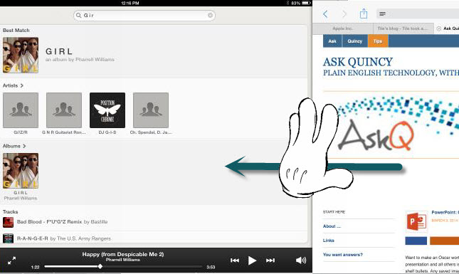
*also a release mechanism to cope with road-rage.
Give your Home button a rest. Gesture (five-fingered** swipe) left or right to get back to your previous apps.
**(four fingers, for Disney execs)
Want to make your spreadsheet more legible? Indents, added where appropriate, will make your spreadsheet easier to mentally digest. Sadly, it won’t make bad financial news easier to swallow.
Watch this 15 second video to learn the what you need to know.
Indent a cell
Select the cell(s) to indent
On the Home tab, in the Alignment Group, click the dialog launcher
(or press CTRL + SHIFT + F to display the Font dialog and click the Alignment tab).
In the Text alignment section, click the Horizontal drop-down and select Left (Indent).
In the Indent field, type or select preferred indent increment (i.e., 1, 2).
Want to make an Oscar worthy, award-winning presentation? The difference between your presentation and all others is design and style. Don’t limit yourself to cookie-cutter, off the shelf bullets. Any saved image can be a source for better bullets.
Watch this 60 second video to learn all you need to know
Select text to be formatted.
On the Home tab, in the Paragraph group, click the Bullets drop-down and select Bullets and Numbering. The Bullets and Numbering dialog appears.
Click Picture. The Picture Bullet dialog appears.
Click Import. A file browser window opens.
Navigate to saved image file (i.e. JPG, GIF) and select picture.
Click Add. The image is added to the picture gallery.
Sparklines are an easy way to add visual trend-lines to your tabular data. And what better way to distract your audience than by dangling something sparkly in front of them!
Watch this 60 second video to learn the what you need to know.
Inserting Sparklines to your Excel data
On the Insert tab, in the Sparklines group, click Sparkline type (e.g., Line). The Create Sparklines dialog appears.
In the Data Range field enter the values to be charted.
In the Location Range field enter cell range where char is to be displayed.
Click OK.
Tip:With an inserted sparkline selected, the Sparklines Tools: Design tab appears on the Ribbon. Use the tools on this tab to change colors and add markers.
Has Valentine’s day snuck up on you this year? Are you buried under too much snow to card shop? Borrow from Microsoft’s templates. Word and PowerPoint have hundreds of print-ready and animated templates to choose from.
Word 2013 TemplatesPowerPoint 2013 Templates
To Download and Create a Valentine
In either Word or PowerPoint, click File tab and select New.
In the Search bar enter Valentine and press Search icon.
Whitespace (or any other background color) can make your inserted images look like a kindergarten stickers. Solution: remove unwanted colors using Set Transparency.
Watch this 60 second video to learn all you need to know
Select the picture or image to be edited.
On the Ribbon, click on the Picture Tools: Format tab.
In the Adjust group click Color (or Recolor, in version 2007) and select Set Transparent Color.
On the selected image, click on the color to remove (i.e. make transparent). That color is erased from the selected image.
Its well past the new year so a littlebubbly is long overdue. Bubble charts are great in that they allow you to graph in 3 dimensions: Length, Height and Breadth (or area). Although the steps below are written with Excel in mind, they can also be applied to PowerPoint.
Watch this 3½ minute video to learn the basics regarding interpreting and creating bubble charts.
Creating a Bubble Chart
Input your data, placing the X-axis data in the first column, Y-axis data in the second column, and the area (bubble size) in the third column.
Select the data.
On the Insert tab, in the Chart group, Click XY and select from Bubble types. A Bubble chart is added to the worksheet
Note: If necessary click Switch Row/Column (on the Chart Tools:Design tab) to swap the series data.
Adding Data Labels
CLICK on one of the bubbles in the series. The entire series becomes selected.
RIGHT+CLICK one of the selected bubbles and select Add Data Labels. Data labels will appear.
To format label appearance and content, RIGHT+CLICK on a bubble and select Format Data Labels.
Formatting the Bubble Appearance (Fill)
CLICK on one of the bubbles in the series. The entire series becomes selected..
CLICK (again) on the bubble. The single bubble will be selected.
RIGHT+CLICK on the selected bubble and select Format Data Point. The Format Data Point dialog/pane appears.
Select Fill and set the fill options (e.g., color, pattern, fill, etc).